13.2 Examples of Flooding Events
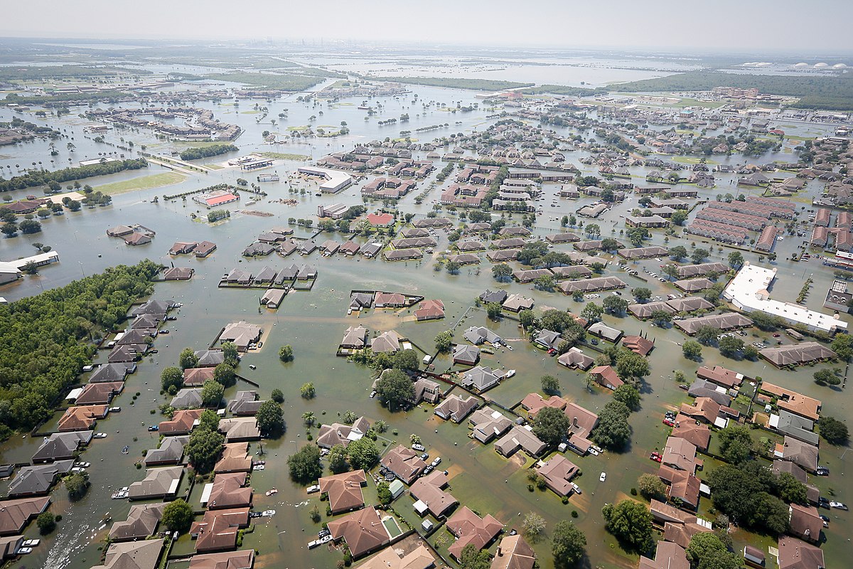
In late August of 2017, Category 4 Hurricane Harvey made landfall near to Corpus Christi, Texas, and then slowly moved east, remaining almost stationary over the Houston region for several days. In that time more than 1000 mm of rain fell over a large area. There was widespread flooding (Figure 13.2.1), more than 100 people died, and the amount of damage is estimated to have been $125 billion, mostly in the form of damages to buildings. In terms of the aggregate rainfall amount measured, Harvey was the wettest tropical storm ever to affect the United States. For a majority of the stream gauging stations analyzed in the region by the USGS, the peak discharges during Harvey were the highest on record.[1]
As we’ll see in Chapter 15, the annual number of tropical storms in the Atlantic basin has been increasing in recent decades, mostly as a result of increased ocean water temperatures as the climate has warmed. The higher water and air temperatures also mean that more water is transferred from the ocean to the atmosphere as a tropical storm evolves, and so we can look forward to a future with more very wet systems like Harvey to cause flooding.
Most streams in Canada and the northern US have the greatest risk of flooding in the late spring and early summer when stream discharges rise in response to melting snow. In some cases, this is exacerbated by spring rainstorms. In years when melting is especially fast because of a sudden rise in temperature, and/or spring storms are particularly intense, flooding can be very severe.
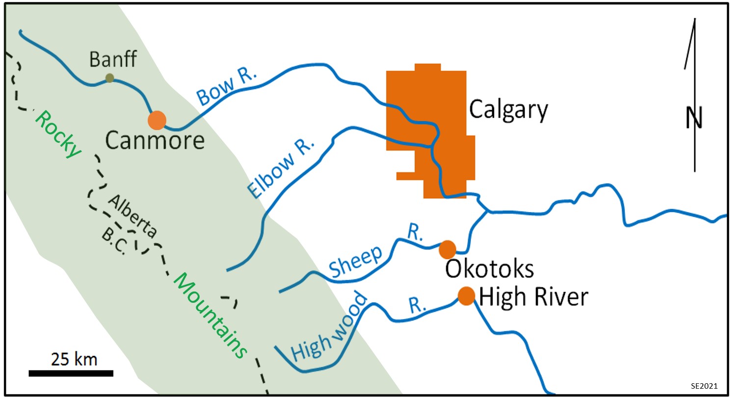
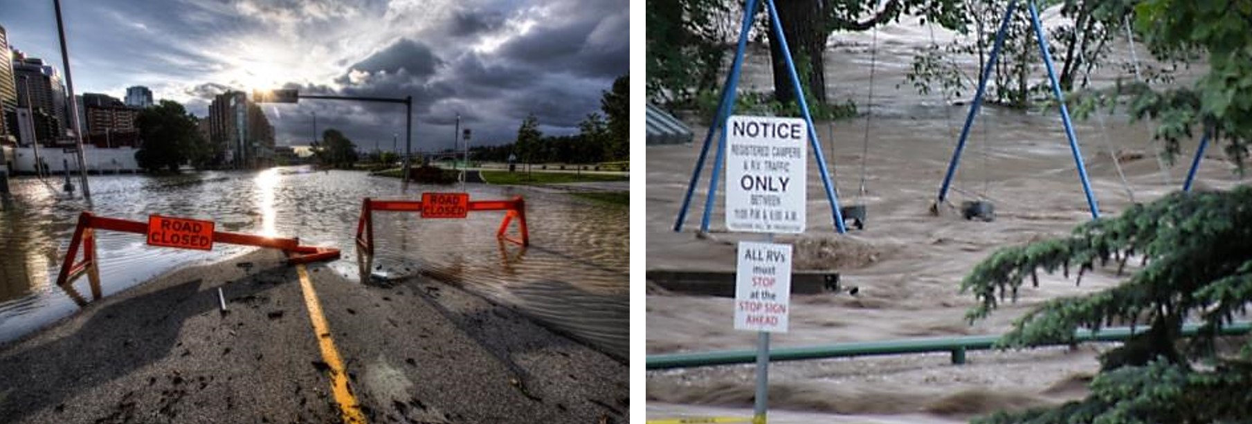
Serious flooding in Alberta in June of 2013 was initiated by rapid snow melt in the Rocky Mountains and was worsened by heavy rains due to an anomalous flow of moist air from the Pacific. Rainfall amounts exceeded 200 mm in 36 hours at Canmore and 325 mm in 48 hours at High River (Figure 13.2.2). The discharges of several rivers in the area, including the Bow River in Banff, Canmore and Calgary, the Elbow River in Calgary, the Sheep River in Okotoks and the Highwood River in High River, reached levels that were 5 to 10 times higher than normal for the late June. Large parts of Calgary, Okotoks and High River were flooded, and 5 people died (see Figure 13.2.3). The cost of the 2013 flood is estimated to have been approximately $5 billion, making it the most expensive flood event in Canadian history.
The Himalayan region is a common source of snow-melt flooding in China, India, Pakistan, Bangladesh, and other countries in the region, but there have also been many slope-failure related floods in the mountains. In July 2000, a slope-failure in China dammed up the Satluj River, forming a temporary lake. By July 31st the water level in the lake had risen enough to flow over and then quickly erode the dam, releasing a massive flood that is said to have increased the water level of the river by 20 metres. Over 150 lives were lost, 250 houses destroyed, and 20 km of road and 7 bridges washed out. As many as 1000 irrigation, sewerage, flood protection, power installations and water supply systems were damaged.[2]
Estimating Flood Probability
Providing that we have enough stream discharge data from previous years it is possible to estimate the probability that a flood of a certain size will happen at some time in the future. Flood probability is determined by calculating the recurrence interval (Ri), the estimated average time between events of a particular discharge, for any given stream. This type of information is useful for planners that have to make decisions about approving proposals for infrastructure projects (buildings, roads etc.) within flood plains, and also for anyone that wants to live near to a river. The recurrence interval for any particular flood magnitude can be estimated using the equation:
Ri = (n+1)/r
where n is the number of years for which maximum discharge levels are known, and r is the rank of the flood level that we want to assess (the biggest flood on record is ranked 1, the second biggest ranked 2, etc.).
By way of example, Figure 13.2.4 shows the record of maximum discharges each year on the Bow River at Calgary between 1915 and 2018. The number of data points (n) is 104. The biggest flood (therefore with r = 1) during that period was the one in 2013, with a maximum discharge of just over 1800 m3/s. Using the equation: Ri = (n+1)/r, we get Ri = (104+1)/1, which means that Ri = 105, so the estimated recurrence interval for a flood of that size is 105 years. The probability of such a flood in any future year is 1/Ri, which is 0.96%. In other words, there is a 1% probability of another large flood (like 2013) next year, or in ten years. The fifth largest flood was just a few years earlier in 2005, at 791 m3/s. Ri for that flood is (104+1)/5 = 21 years. The recurrence probability for a flood of that size is 4.8%. You can try this out with some different numbers in Exercise 13.1.
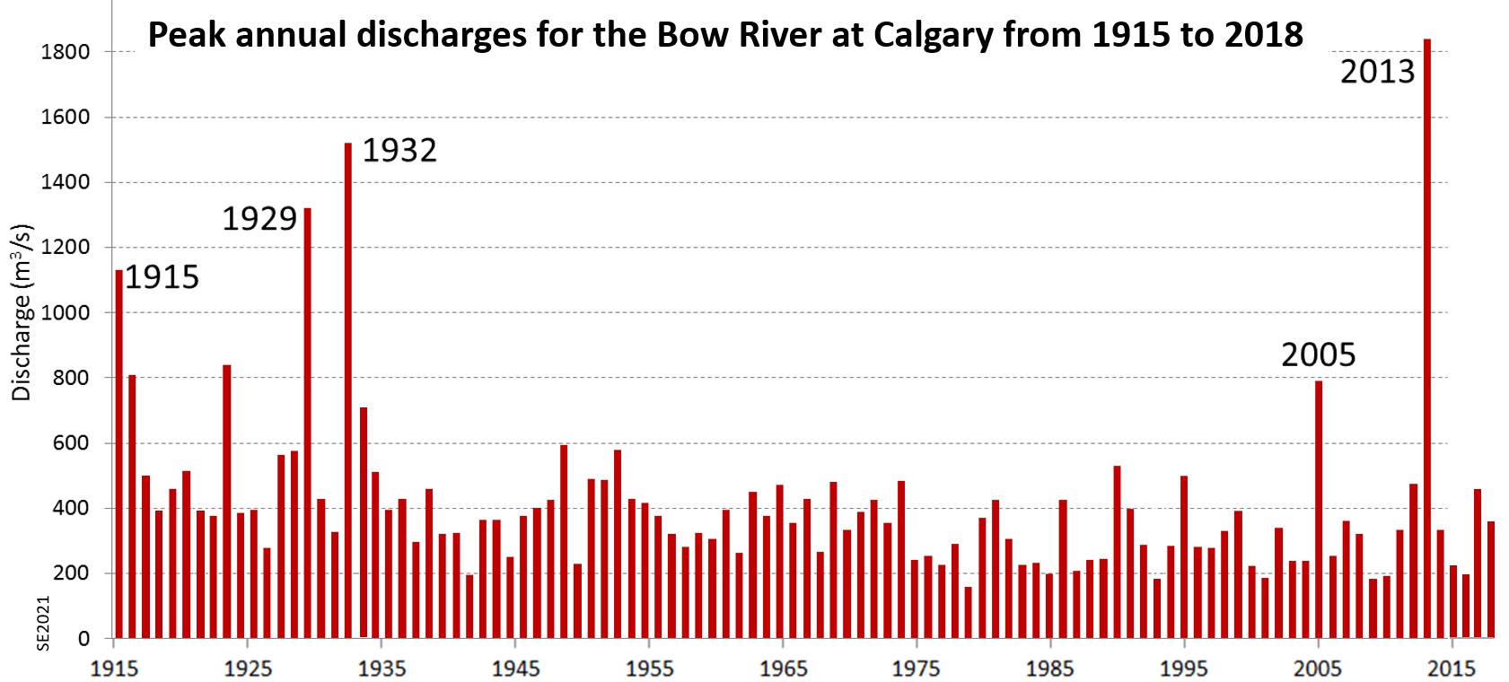
One of the things that the Bow River flood record teaches us is that we although we can determine a flood probability, we can’t actually predict when there is going to be a big flood, nor how big it will be, so in order to minimize damage and casualties we need to be prepared. Some of the ways of doing that are as follows:
- Mapping flood plains and not building within them,
- Building dykes or dams where necessary,
- Monitoring the winter snow pack, the weather, and stream discharges,
- Creating emergency plans, and
- Educating the public.
Emergency measures organizations use calculations of Ri to report past, current or predicted floods using terms like “100-year flood”. That means that the flood was, or is expected to be, as big as any flood in the past 100 years. Of course such calculations are only as good as the amount of data available, and the quality of those data.
Another important point to remember is that estimation of flood probabilities based on past data relies on the premise that the climate conditions and land-use patterns that produced the historical record are still relevant in the future. As we know, our climate has changed quite dramatically over the past several decades, and that may have changed the climate factors, such as likely storm intensity, snow accumulation amounts, timing and rate of thawing etc., so that premise is not valid. Furthermore, land use changes may have changed the way water runs off the surface, and that could also change the probability of future large floods.
Exercise 13.1 More Bow River Flood Probabilities
Using the data for the Bow River in Figure 13.2.4 and using the formula Ri = (n+1)/r, (where Ri is the recurrence interval, n is the number of years for which maximum discharge levels are known (104 in this case), and r is the rank of the flood level that we want to assess (the biggest flood on record is ranked 1, the second biggest ranked 2, etc.)) is do the following:
- Calculate the recurrence interval for the 2nd largest flood (1932, 1520 m3/s).
- What is the probability that a flood the size of the 3rd largest (1320 m3/s in 1929) will happen next year?
- Examine the 104-year trend for floods on the Bow River. If you ignore the major floods (the labelled ones), what is the general trend of peak discharges over that time?
Exercise answers are provided Appendix 2
Media Attributions
- Figure 13.2.1 Support During Hurricane Harvey from South Carolina National Guard, 2017, public domain image via Wikimedia Commons, https://commons.wikimedia.org/wiki/File:Support_during_Hurricane_Harvey_(TX)_(50).jpg
- Figure 13.2.2 Steven Earle, CC BY 4.0
- Figure 13.2.3 (left) Riverfront Ave Calgary Flood by Ryan L. C. Quan, 2013, CC BY SA 3.0, via Wikipedia, https://en.wikipedia.org/wiki/2013_Alberta_floods#/media/File:Riverfront_Ave_Calgary_Flood_2013.jpg; (right) Okotoks June 20 by “Stephanie N. Jones” (Jadelicia), 2013, CC BY SA 3.0, via Wikimedia Commons, https://en.wikipedia.org/wiki/2013_Alberta_floods#/media/File:Okotoks_-_June_20,_2013_-_Flood_waters_in_local_campground_playground-03.JPG
- Figure 13.2.4 Steven Earle, CC BY 4.0, based on Open Government License – Canada data at Water Survey of Canada, Environment Canada, https://wateroffice.ec.gc.ca/
_(50).jpg)
- Watson, K. et al. (2018). Characterization of peak streamflows and flood inundation of selected areas in southeastern Texas and southwestern Louisiana from the August and September 2017 flood resulting from Hurricane Harvey. USGS Scientific Investigations Report 2018-5070. https://doi.org/10.3133/sir20185070 ↵
- Gupta, V. & Sah, M. (2008). Impact of the Trans-Himalayan Landslide Lake Outburst Flood (LLOF) in the Satluj catchment, Himachal Pradesh, India. Natural Hazards 45, 379–390. https://doi.org/10.1007/s11069-007-9174-6 ↵